
Acre by Acre
Scientists combine old and new procedures to map Texas vegetation.
By Rae Nadler-Olenick
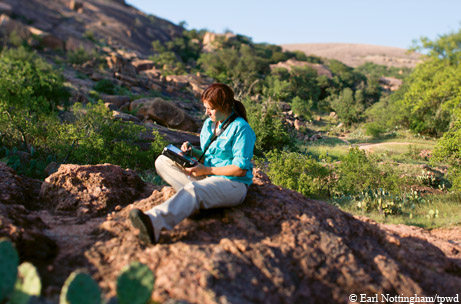
The white Texas Parks and Wildlife Department truck, equipped with powerful GPS gear and a sturdy road-worthy laptop mounted next to the steering column, rolls along Still Road in Blanco County, near the junction of the Edwards Plateau and the Llano Uplift. Behind the wheel is plant ecologist Amie Treuer-Kuehn.
“Typically, what I do is drive along remote county roads, stopping every mile to see what I can see,” she says. “If after four or five miles I keep seeing the same landscape, I’ll move on to somewhere else.”
Treuer-Kuehn is “ground truthing” — identifying and recording the vegetation patterns characteristic of Texas’ 254 counties through personal observation. The information will later be correlated with data from a satellite.
Her work is part of a five-year survey whose ambitious goal is to map the vegetation systems of Texas with unprecedented accuracy. It supersedes TPWD’s pioneering Vegetation Types of Texas project, conducted between 1974 and 1984 and now outdated.
The present survey, begun in 2007, is more than halfway complete, with Treuer-Kuehn putting in long days on the road — sometimes three weeks a month — and painstakingly entering her observations into her notebook computer to be uploaded to the project servers later. So far she’s covered close to 200 counties. The finished map will incorporate detailed biological and ecological data on several hundred Texas ecological systems, from shrubland to forest to prairie to swamp.
She stops at a roadside stretch of low shrub growth dotted with small live oaks and ashe junipers, a handful of dead hackberries and the occasional Texas persimmon.
“This looks like typical Edwards Plateau, but you can tell it’s been grazed by the size of the trees and by the amount of prickly pear and other stuff cattle won’t eat,” she explains, scanning an area approximately 100 meters on a side (one hectare). “I’d call it a shrubland, based on the fact that I see probably 26 percent shrubs.”
For purposes of the survey, woody plants over 15 feet high are classified as trees; under 15 feet, as shrubs. An ecosystem is named for the vegetation types that cover more than 25 percent of the total area.
Later on, Treuer-Kuehn demonstrates the versatility of her mobile computer setup. The notebook has been loaded with satellite imagery and with the digitized Geologic Atlas of Texas, enabling her to identify the geological features of any coordinate. Once she’s categorized the dominant plant species, she sets her data point, and a data entry form pops up. She’ll take a photograph of the area for a visual record, then move on to the next observation spot.
The ubiquity of wireless computer access allows her to upload her data from the field — often from her hotel room at night. It’s a fast, easy process compared to the last time around.
Upon receiving her output, project personnel will enter it into a computer model along with detailed information about the locality’s soils, geology and physical landscape.
Then they’ll crunch all those numbers together to yield a color-keyed picture of the local vegetation.
“We’re standing on the shoulders of what others did before,” says geographic information system (GIS) lab manager Kim Ludeke. “That’s the bigger part of the story.”
The story begins back in the mid-1970s, with the foresight of one man, the late Craig “Pepper” McMahan, who was director of TPWD’s Wildlife Division.
“He was a visionary, a Texan deeply committed to conservation in Texas who grappled with huge problems,” recalls Carl Frentress, the project’s first recruit, who served as project leader through the crucial first three years of development and the production of the first map.

The time was propitious. NASA’s first Landsats were circling the globe, collecting information about Earth’s surface geography. NASA — in search of applications for its new technology — made the information freely available. And Gov. Dolph Briscoe, eager to catch the bandwagon, had established an Office of Information Services to facilitate remote-sensing projects in Texas.
McMahan envisioned using that wealth of imaging data to create a detailed statewide map of Texas habitat. Such a map, he knew, would be invaluable for long-range planning of the division’s large-scale wildlife management programs.
His proposal proved a perfect fit. Obtaining grant money through the governor’s program, he assembled a team. For biological expertise, he tapped Frentress and Roy Frye, both TPWD wildlife biologists then engaged in avian field studies elsewhere. His chosen computer specialist, Don McCarty — whose educational background included both marine biology and computer science — was already in Austin, working as a programmer and statistical analyst in TPWD’s business department.
As Landsat passed over Texas every nine hours (there were two satellites, each requiring 18 days to retrace the same spot on Earth’s surface), its light and infrared sensors gathered information on the state’s ground cover. The data was then downloaded to NASA and saved in digital form on nine-track magnetic tape. The team’s challenge was to convert that digitized information into a color-coded map of Texas’ principal vegetation zones.
Considerable preparation went into the venture. Frentress and Frye attended several months of specialized technical classes offered locally through the governor’s office, and they traveled to NASA’s Earth Resources Technology Lab in Mississippi for hands-on practice with the hardware they’d be using. McCarty, already tech-savvy, would join the team the following year, when the data analysis phase began.
McCarty’s former colleagues all laud his computer wizardry. “He was the guy behind the scenes who did all the technical work,” says Frye. “Without him, there wouldn’t have been any maps.”
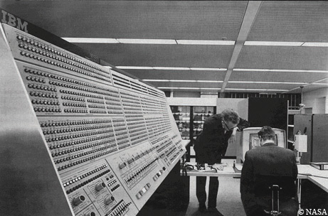
NASA, McCarty recalls, contributed two kinds of vital information. There were the nine-inch tape reels on which the data was stored. And there was the collection of computer programs known as Patrec (pattern recognition) that turned the raw data into pixels on a screen. The latter came “in the form of about five boxes of IBM punch cards.” Worse, they were coded for a different computer than the IBM-360 that TPWD used.
McCarty plunged into the herculean task of rewriting NASA’s computer code, designed for a Varian data machine, to run on an IBM-360. Translating the Fortran and assembly languages into PL-1 required close collaboration with NASA.
“I was on the phone with them for hours,” he says. “I spent a lot of time on the phone.”
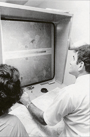
Meanwhile, TPWD had acquired a piece of custom-built, state-of-the-art equipment — identical to the one NASA used — capable of displaying downloaded satellite data in a graphical format. Dubbed PIDS (portable image display system), the three-tiered instrument converted digital information to a colored cathode ray tube (CRT) display. The bottom section held data tape reels. The middle housed the wiring that communicated with the remote IBM mainframe. A color TV monitor perched on top.
Remote ground cover mapping works on the principle of reflectance: Different types of vegetation reflect different amounts of the sun’s radiation. As Landsat passed overhead scanning the landscape, it would capture the reflectance at four separate wavelengths for every 1.1 acres of land. The computer read the tapes, broke down the stored data according to wavelength intensity, translated it into a range of visible colors using complex statistical analysis methods and displayed the results on the CRT screen, where each pixel represented approximately an acre.
But the display system had to be “trained” to display its results in an identifiable format. That meant finding sizable, well-represented swaths (training fields) of each desired vegetation type on the ground, then matching them one-on-one with their counterpart patterns on the PIDS screen. Guided by tips from local botanists, armed with county highway maps, county aerial photographs supplied by the U.S. Department of Agriculture and data sheets, the ground-truthers set out into the field.
Frye spent the most time ground-truthing. He describes the process — before GPS technology came along:
“We knew what vegetation types we wanted to map in an area before we started,” Frye says. “I’d drive out there and find field-representative sites for each one. Say we wanted to map bottomland hardwoods in southeast Jasper County. I’d go down the road, and if I found a good spot, I’d have to have a road intersection close by so that I knew where I was. I’d write that information down on data sheet and on the aerial photograph.”
Once back at the office, he and his colleagues would carefully match each photograph to its position on a satellite data picture displayed on the screen. The collection of reflectance values associated with a given position on the screen became a unique “signature” — recognizable to the computer — for the vegetation type associated with that position. It also corresponded to a specific color or colors.
Kirby Brown joined the project in its fourth year after Carl Frentress left to return to his first love, fieldwork. Brown arrived fresh from graduate school at Texas A&M University bearing credentials in both wildlife studies and remote sensing.
“Knowing, say, that this was an oak woods, we’d grab those reflectivities and run the computer overnight to highlight everything in the image that was in that reflectivity,” Brown says. “Then we’d turn around and ground-truth that, going back into the field to see if we could replicate it in a different place.”
Sometimes they couldn’t, and parameters had to be adjusted and data rerun. “They weren’t very happy about that in the computer room,” he adds.
In the computer room, McCarty presided over the processing of the tapes. Among his many tasks were creating the signature files for each vegetation type and creating the map projections by which the information would be displayed.
He also developed a time-saving way to overlay data from two separate seasons: spring and winter. The computing process, he explains, was extremely time-consuming back then. Most of the number-crunching took place at night because the computer was needed for business applications during the day. In fact, he frequently spent the night there.
“I felt sorry for him,” Frye recalls, but McCarty says he didn’t mind at all.
Fast-forward to 2010. Gone are the IBM punch cards, the tape spindles, the antiquated display console. Today, NASA’s raw data can readily be downloaded directly from the satellite to personal computers no larger than the Dell workstation on Duane German’s desk. German, a field ecologist turned project manager, coordinates the current mapping project. A more recent Landsat rules the sky, and powerful new technology has made possible many refinements undreamed of 25 years ago.
Today’s maps encompass soil, geography and geology data as well as vegetation. They combine three seasons (winter, spring and fall) instead of two (winter and spring) and utilize six wavelengths as opposed to four. Screen resolution has gone from more than an acre to 10 meters. And a new classification system has brought the number of identified ecosystems from the original 57 to several hundred.
Also new is the decision to farm out much of the technical operations.
“We could have built an in-house team from scratch that might not be needed when the project ended in a few years,” German explains. “Or we could enlist a facility that already has trained personnel in place.”
They chose the Missouri Resources Assessment Partnership (MoRAP), a University of Missouri-affiliated research center based in Columbia, Mo., and headed by a one-time Texas Parks and Wildlife Department staff member. David Diamond, its director, is a Ph.D. ecologist who during his eight-year stint at TPWD came to know several members of the earlier mapping team, including McMahan, Frye and McCarty.
Working with him at MoRAP is Lee Elliott, another ecologist with extensive Texas field experience.
“Both of us have a long history of this kind of work,” Diamond explains. “It kind of takes a technical hand and ecological expertise. We have both of those.” Clayton Blodgett, who’s in charge of remote sensing on the project, and information security specialist Diane True, who combines all the information into the final digital maps, round out his group.
The new maps have already found successful applications. The Texas Forest Service uses them to do fire modeling for controlled burns and to pinpoint areas ripe for restoration efforts of species like longleaf pine. The U.S. Fish and Wildlife Service makes use of them for fire risk assessment.
Kirby Brown, now vice president for public policy for the Texas Wildlife Association, points out that one of the original survey’s goals was to track changes in habitat at 10-year intervals.
“Having it done now is very important,” he says. “I think we’re going to show an amazing group of changes.”